Joyful noise
I’ve been seeing lots of folks talk about AIOr, as an aging scientist would say, machine learning. as if only a few blessed humans could understand it. I think you need some fundamentals and some time messing around with models. Once you have both, parts of it get almost annoyingly predictable. One of those fundamentals is noise outsourcing: write the random thing you care about as a function of noise.
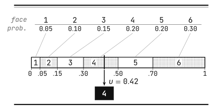
Let’s start with our old friend, the loaded die. Its faces are weighted $(0.05,\;0.10,\;0.15,\;0.20,\;0.20,\;0.30)$. From that list you can work out the mean roll or the die’s favourite face. How do you get the computer to roll it?
There’s a library call for this, of course. Let’s ignore it and obsess over the question a little bit.
We’ll allow ourselves exactly one treat: a function that returns a number $U$ drawn uniformly from $[0,1)$. We’ll look at where that draw comes from at the end.
To roll the die, cut the unit interval into six pieces whose lengths are the six probabilities,
\[[0,.05),\quad [.05,.15),\quad [.15,.30),\quad [.30,.50),\quad [.50,.70),\quad [.70,1),\]draw a number, and report which piece it fell in. A draw of $0.42$ rolls a four, and $0.91$ rolls a six. The chance of landing in a piece is its length, which is exactly the probability we gave that face.
What I love here is how little of the algorithm is random. Once you draw the noise (the random number), everything else is a lookup. Pass that number in as an argument and the roll becomes an ordinary deterministic function.
The same setup shows up in language models and diffusion models. A language model spits out probabilities for the next token. A sampler uses a random draw to pick one, much like rolling the die. A diffusion sampler starts from noise and nudges it, little by little, into something that looks like data.
Giving randomness an input
Write $U$ for the uniform draw and $f$ for the interval lookup, so the simulated face is
\[Y=f(U),\qquad U\sim\operatorname{Uniform}[0,1).\]It’s easy to confuse $f$ with the probability mass function of $Y$. The mass function gives you the probability of each face. The sampler $f$ gives you a face for each noise value $u \in \text{supp}(U)$.
For any finite distribution $p_1,\ldots,p_K$, take cumulative sums
\[c_0=0,\qquad c_k=\sum_{j=1}^k p_j,\]and set $f(u)=k$ whenever $c_{k-1}\le u<c_k$. Then
\[P(f(U)=k)=P(c_{k-1}\le U<c_k)=c_k-c_{k-1}=p_k,\]and that’s the entire proof. In pseudocode, assuming the probabilities sum to 1:
sample_category(probabilities, u):
    cumulative = 0
    for category, probability in probabilities:
        cumulative += probability
        if u < cumulative:
            return category
The caller passes in u, so we can test a particular case or run the sampler twice with exactly the same noise.
Now let the probabilities depend on some context $x$, say, which of several loaded dice we’re holding. Replace $p_k$ by $p_k(x)$ and the boundaries shift. The lookup works the same way:
\[Y=f(X,U),\qquad U\sim\operatorname{Uniform}[0,1),\qquad U\perp X.\]The $\perp$ means independence: whatever the context, the noise is a fresh uniform draw. The context sets the boundaries and the noise decides where we land. If $U$ could depend on $X$, we could smuggle the whole sampling problem into the noise source and call it solved.
“Noise” is a slightly unfortunate word, by the way. It needn’t mean measurement error. It’s the randomness we feed the sampler, even if all we do with it is pick a face.
From intervals to distributions
The interval trick gives us a general recipe for checking whether a sampler is right. Pick any set of outputs $A$, collect all the inputs $u$ that land in it, and measure how likely it is to draw one of them:
\[P(f(U)\in A)=P\bigl(U\in\{u:f(u)\in A\}\bigr).\]Since our noise is uniform, “how likely” is just a length. For the die, the inputs that roll an even face add up to $0.10+0.20+0.30=0.60$ of the interval, which is exactly the probability of an even face. The resulting distribution is the pushforward of the noise through $f$. What I like about it is that we only need the noise distribution and the function to define the output distributionA diffusion sampler can define a distribution over images without anyone writing down its density. .
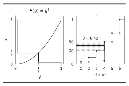
For a real-valued variable, the cumulative distribution function (CDF) is $F(y)=P(Y\le y)$. It goes from 0 to 1 as $y$ grows. Pick a random height $u$ between 0 and 1 and move from left to right until the CDF reaches or exceeds that height. That’s your sample. For $0<u<1$, the quantile function is
\[Q(u)=\inf\{y:F(y)\ge u\}.\]If $F$ is continuous and strictly increasing, $Q$ is just $F^{-1}$. The $\inf$ is there so the definition still works when $F$ has jumps (discrete outcomes) or flat stretches (gaps with no mass). The die’s CDF looks like a staircase. Each jump hands one face a whole band of heights. The width of that band is the face’s probability, so we get our intervals back.
Fix a threshold $y$. The quantile $Q(u)$ lands at or below $y$ exactly when $u\le F(y)$, so
\[P(Q(U)\le y)=P(U\le F(y))=F(y).\]The output has the right CDF, hence the right distributionSome fine print: $Q(0)$ can be anything because an ideal uniform draw hits any single point with probability zero. That’s also why we can put the interval boundaries on either side in the die example. Computers are finite and sometimes annoying. They’ll make us care about endpoints again. .
Take $F(y)=y^2$ on $[0,1]$. Then $Q(u)=\sqrt u$, so to sample from it we draw a uniform number and take its square root. The output leans toward larger values: every $u$ above $1/4$ gives a sample above $1/2$, so that happens with probability $3/4$.
Conditioning on context works just like it did for the die. For each context $x$, use its own CDF,
\[F_x(y)=P(Y\le y\mid X=x),\qquad f(x,u)=Q_x(u),\]and the same $f$ can produce a point mass for one $x$ and a distribution with several peaks for another. The noise stays the same boring uniform.
How far does this go?
The general result goes by noise outsourcing (or the randomization lemma). For random variables $X$ and $Y$ in standard Borel spaces, there’s a measurable function $f$ such that
\[(X,Y)\stackrel{d}{=}(X,f(X,U)),\qquad U\sim\operatorname{Uniform}[0,1),\qquad U\perp X,\]where $\stackrel{d}{=}$ means equality in distribution: both pairs assign the same probability to every measurable eventThere’s a stronger version with $Y=f(X,U)$ almost surely, possibly on an enlarged probability space. Here $U$ is still independent of $X$, but we choose it jointly with $Y$ rather than make a fresh draw. See Austin, Lemma 3.1. .
“Standard Borel” sounds scary, but it covers pretty much anything we’d call data: finite labels, integers, real vectors, images as arrays, finite strings. We can measurably encode any such space into the unit interval. That lets us use the quantile trick again: encode the outcomes as real numbers, sample from the encoded distribution, and decode the result. Doing this consistently across contexts takes some care, but no new randomness.
Measurable roughly means that for any measurable set of outputs, we can assign a probability to the inputs that land there. The theorem tells us a function like this exists. It doesn’t say what function this is, whether we can compute it, let alone learn it or run it quickly.
One thing bugged me the first time I saw this: how can a single random number carry enough randomness for a whole image, or even for two independent numbers?
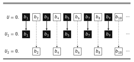
An ideal uniform real has infinitely many binary digits,
\[U=0.b_1b_2b_3b_4\ldots,\]and those digits are independent fair coin flipsAny specific prefix of $n$ bits picks out an interval of length $2^{-n}$, so every prefix is equally likely. We’re ignoring numbers with two binary expansions, like $0.0111\ldots=0.1000\ldots$, which have probability zero. . So we can deal the odd digits to one number and the even ones to another,
\[U_1=0.b_1b_3b_5\ldots,\qquad U_2=0.b_2b_4b_6\ldots,\]and get two independent uniforms. Split the positions into more subsequences and you get as many as you want. This is the magic trick: The single number $U$ in the theorem is an infinite tape of random bits, way more than a floating-point number in a register could ever hold.
In code, it’s cleaner to make the noise argument a vector or a stream, but the idea is the same: put every random choice in that argument, and once the stream is fixed, even a program that asks for fresh randomness halfway through is deterministic. It’s just reading further down the tape.
Making Gaussian noise
Suppose we want two independent standard normals. Their joint density
\[p(z_1,z_2)=\frac{1}{2\pi}\exp\Bigl\{-\frac{z_1^2+z_2^2}{2}\Bigr\}\]only depends on the distance from the origin. Since it looks the same in every direction, we can pick an angle uniformly around the circle and then pick a radius. The angle is easy: $\Theta=2\pi U_2$.
The radius takes a bit more thought. A thin ring at radius $r$ has circumference $2\pi r$, so it holds more area than a ring of the same width closer to the origin. Its probability is roughly density times area,
\[\frac{1}{2\pi}\exp\{-r^2/2\}\cdot 2\pi r\,dr =r\exp\{-r^2/2\}\,dr,\]so the radius has density $r\exp{-r^2/2}$ for $r\ge0$. Integrating from $r$ outward gives a surprisingly clean tail,
\[P(R>r)=\int_r^\infty s\exp\{-s^2/2\}\,ds=\exp\{-r^2/2\},\]which we can invert by hand. For a uniform $U_1$, set
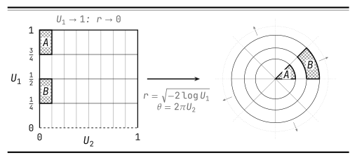
\[R=\sqrt{-2\log U_1}.\]For $r\ge0$, the event $R>r$ is the same as $U_1<\exp{-r^2/2}$, which has exactly the probability we want. With independent $U_1$ and $U_2$ we get an independent radius and angle. Back in Cartesian coordinates,
\[Z_1=\sqrt{-2\log U_1}\cos(2\pi U_2),\qquad Z_2=\sqrt{-2\log U_1}\sin(2\pi U_2).\]This is the Box–Muller transformThe joint density of radius and angle is $r\exp{-r^2/2}/(2\pi)$. Dividing by the polar area factor $r$ gives back the Cartesian density. It factors into a standard normal in each coordinate, so we get normality and independence at once. .
We used a uniform point in a square to pick a Gaussian point in the plane. Equal areas in the square carry equal probability, but they can map to very different areas in the plane. Near the origin, the map squeezes probability into a small region. Far away, it spreads the same amount over a larger one. It’s a pushforward again, just with geometry instead of labeled intervals.
The logarithm needs $U_1>0$. An ideal uniform draw hits zero with probability zero, so we can define the transform there however we want. A real generator can return exactly zero. If your routine returns values in $[0,1)$, using 1 - uniform_0_1() gives you $(0,1]$ and avoids the problem.
Once we have a standard normal $Z$, conditional Gaussians are one line away:
\[Y=\mu(X)+\sigma(X)Z,\qquad Z\perp X.\]The mean and standard deviation can come from a table, a physics model, or a neural network. For vectors, $Y=\mu(X)+L(X)Z$ with $Z\sim\mathcal N(0,I)$ has conditional covariance $L(X)L(X)^\top$. Given $X$, the output coordinates can be correlated even though the noise coordinates are independent. The matrix $L(X)$ can mix them.
A large sampler made of small ones
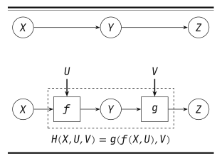
Now let’s chain samplers. Say we first sample $Y$ given $X$, and then $Z$ given $Y$. As programs,
\[Y=f(X,U),\qquad Z=g(Y,V),\]with $U$ and $V$ independent of each other and of $X$. Plugging one into the other,
\[Z=g(f(X,U),V),\]so the whole process is a deterministic function of the context and two noise inputs. If we wanted the distribution of $Z$ as a formula, we’d have to sum or integrate over $Y$, which can be painful. To draw a sample, we run the functions in order.
To see why we use independent noise, take $Y=\mathbf 1{U<1/2}$. The indicator $\mathbf 1$ is one when its condition holds and zero otherwise, so $Y$ is a fair coin. Apply the same test to an independent $V$ and we get a second, independent coin $Z$. Reuse $U$ instead and we get $Z=Y$ every single time. Putting all the randomness on one tape doesn’t mean every step reads the same spot on it.
An autoregressive language model predicts each token from the prompt and the tokens so far. Let $X$ be a prompt and $Y_1,\ldots,Y_n$ the generated tokens. For a fixed length $n$, the model’s joint distribution factors as
\[p_\theta(y_1,\ldots,y_n\mid x) =\prod_{t=1}^n p_\theta(y_t\mid x,y_{<t}),\]where $y_{<t}$ is everything before position $t$ and $\theta$ are the learned parameters. At each step, the network computes a probability vector over the vocabulary, and the sampler turns that vector into a token.
We already know how to do that last part: give each token in the vocabulary an interval as long as its probability, and draw a fresh uniform,
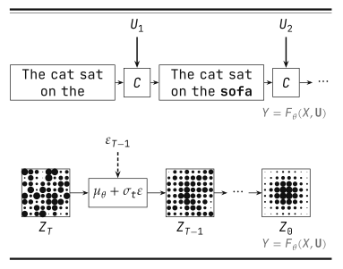
\[Y_t=C\bigl(p_\theta(\cdot\mid X,Y_{<t}),U_t\bigr),\]where $C$ is our categorical sampler from before. Say the prompt is “The cat sat on the” and our imaginary model gives “mat”, “sofa”, and “roof” probabilities $0.50$, $0.30$, and $0.20$. Then $u_t=0.63$ picks “sofa”. That token becomes part of the context for the next step, which is why one early draw can change every distribution that comes after it.
Repeating this samples exactly the joint distribution above, since the probability of following any given path is the product of the conditionals along it. A stop token or a length limit takes care of variable-length text. Collecting the uniforms into a tape $\mathbf U=(U_1,U_2,\ldots)$, the whole thing becomes
\[Y=F_\theta(X,\mathbf U),\]where $F_\theta$ bundles the network calls, the categorical lookups, and the stopping ruleImplementations can use other categorical samplers, such as the Gumbel-max trick. The interval lookup is exact when the uniform draw and arithmetic are exact. .
The decoder can change the distribution of generated text. Greedy decoding picks the most likely token at each step and leaves the noise tape alone. Temperature, top-$k$, and friends change the probabilities before sampling.
During training, a diffusion model sees data corrupted with different amounts of noise. At generation time it starts from pure noise and applies learned updates to turn it into a sample. To keep the prompt $X$ separate, let $Z_T$ be the initial noisy vector and $Z_0$ the output. A common update is
\[Z_T=\varepsilon_T,\qquad Z_{t-1}=\mu_\theta(Z_t,t,X)+\sigma_t\varepsilon_{t-1},\]with independent standard normal $\varepsilon$’s, also independent of $X$. That’s our conditional Gaussian from before, applied over and over. The original denoising diffusion probabilistic model (DDPM) uses this form without the prompt $X$ and adds no noise at the last step.
Since those Gaussians can come from uniforms (via Box–Muller, say), the whole chain is again a function of the context and a noise tape. Some samplers only need the initial noise. In the deterministic version of denoising diffusion implicit models (DDIM), the later steps add no noise, so with the context fixed, $Z_T$ determines the whole trajectory.
Noise outsourcing says how to represent these samplers. It doesn’t tell us whether either one will produce convincing text or images.
Why the choice of function matters
If we want to learn a sampler, it helps if we can differentiate through it. Suppose $f_\theta$ has parameters $\theta$ and we want to minimize an expected loss,
\[L(\theta)=\mathbb E_U[\ell(f_\theta(U))].\]The distribution of $U$ doesn’t depend on $\theta$. If $f_\theta$ is differentiable and we can swap the derivative and the expectation, we can estimate gradients by sampling $U$ and backpropagating straight through the program:
\[\nabla_\theta L(\theta) =\mathbb E_U[\nabla_\theta\ell(f_\theta(U))].\]For a Gaussian $Y=\mu+\sigma Z$, holding $Z$ fixed gives $\partial Y/\partial\mu=1$ and $\partial Y/\partial\sigma=Z$. That’s the reparameterization trick used to train variational autoencoders with Gaussian latent variables. As Bloem-Reddy and Teh point out, noise outsourcing guarantees measurability. To use the trick, we need more from $f$.
Our categorical sampler shows where this can go wrong. Take a Bernoulli draw, a sample that equals one with probability $p$ and zero otherwise:
\[Y_p=\mathbf 1\{U<p\}.\]For a fixed $u$, nudging $p$ almost never changes the sample, so its derivative with respect to $p$ is zero everywhere except at the jump $p=u$. And yet
\[\mathbb E[Y_p]=p,\qquad \frac{d}{dp}\mathbb E[Y_p]=1,\]so backpropagating through the sample misses the effect entirely. The expectation changes because the boundary moves and sweeps over more noise values, and derivatives taken away from the boundary can’t see that.
For discrete samples, one option is to estimate the gradient using the probability of the sampled outcome, as in REINFORCE. We can also look for a smoother representation or use a loss that avoids differentiating through the sample.
The same distribution can describe different worlds
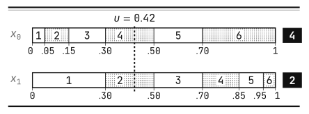
Our loaded die doesn’t care where its intervals sit: move the interval for six to the front, shuffle the rest, and the probabilities don’t change. But now $u=0.42$ might roll a different face.
Evaluating $f(x_0,U)$ and $f(x_1,U)$ with the same $U$ gives a joint distribution over two outputs, called a coupling. Each output has the right distribution on its own. Which outputs go together depends on which $f$ we picked.
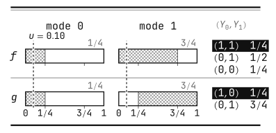
A system has two modes, $x=0$ and $x=1$. Mode 0 succeeds with probability $1/4$ and mode 1 with probability $3/4$. One valid sampler is
\[f(0,u)=\mathbf 1\{u<1/4\},\qquad f(1,u)=\mathbf 1\{u<3/4\}.\]With this one, every $u$ that succeeds in mode 0 still succeeds in mode 1. Another sampler with the same success rates is
\[g(0,u)=\mathbf 1\{u<1/4\},\qquad g(1,u)=\mathbf 1\{u\ge1/4\}.\]The probabilities are still $1/4$ and $3/4$, but now every $u$ that succeeds in mode 0 fails in mode 1. At $u=0.10$, $f$ gives the pair $(1,1)$ and $g$ gives $(1,0)$. Under $g$, the higher success rate comes entirely from turning the old failures into successes.
Both samplers give an average gain of $1/2$. The two success rates alone can’t tell us whether a particular success survives the switch.
A structural causal model gives each variable an equation,
\[V_i=h_i(\operatorname{Pa}_i,E_i),\]where $\operatorname{Pa}_i$ are its direct causes and $E_i$ is the noise from outside the model’s equations. If there are no cycles, we can evaluate each equation after its causes, just like our chained samplers. A causal model assumes that the other equations keep working when we intervene. Setting $V_j=a$ replaces its equation with the constant $a$ and leaves the rest alone. Pearl’s overview of causal inference describes this setup.
With such a model, we can compare interventions while holding the exogenous noise fixed, which is what a counterfactual isFor an observed individual, we first infer what the observations tell us about their noise, and only then run the modified equations. That inference can leave uncertainty, since an observed outcome rarely pins down a unique noise value. .
Our two samplers could be two models of the mode switch. If we assign the mode independently of $U$, both produce the same distribution of observed outcomes and the same success rates when we set the mode directly. To choose between their counterfactual answers, we’d need another assumption, such as whether switching can turn a success into a failure.
Writing a conditional as $Y=f(X,U)$ doesn’t make $X$ a cause of $Y$. We can factor the same joint distribution the other way around and write $X=g(Y,V)$. Taking the noise inputs for different variables to be independent is also an assumption. If we leave out a common cause, those variables may need correlated or shared noise.
Where the uniform comes from
On a regular computer, the uniform draw usually comes from a pseudorandom number generator (PRNG), which is itself a deterministic program. Write its internal state as $S_t$, its transition as $T$, and its output as $O$:
\[S_{t+1}=T(S_t),\qquad J_t=O(S_t).\]A simple way to turn an integer output into a number in $[0,1)$ is
\[U_t=J_t/2^w,\qquad J_t\in\{0,1,\ldots,2^w-1\}.\]The possible values form a finite grid. For $U_t$ to be uniform on it, $J_t$ has to be uniform over those integers. Dividing by $2^w$ won’t fix a bad generator. Python’s random(), for instance, returns multiples of $2^{-53}$ in $[0,1)$, as its documentation explains.
Take the toy rule
\[S_{t+1}=(5S_t+1)\bmod16,\qquad U_t=S_t/16.\]Starting from zero, the states are
\[0,1,6,15,12,13,2,11,8,9,14,7,4,5,10,3,0,\ldots\]Every state shows up exactly once before the cycle repeats. If we start from a uniformly chosen state, every later state is also uniform, since each step permutes the sixteen values. Yet if you see one state, you know the next. A perfect histogram doesn’t mean good randomnessPlease don’t use this generator for anything serious. .
Real generators have much larger states and are designed to avoid patterns that would matter for their intended use. Still, no deterministic generator can create unlimited independent bits from a finite seed. Even if we choose the seed at random, we can get at most as many different streams as there are seeds.
Finite precision also changes the distributions our samplers produce. On a grid of sixteen equally likely points, any deterministic binary sampler succeeds with a probability that’s a multiple of $1/16$, so it can’t hit $0.10$ exactly. Box–Muller applied to finitely many input pairs gives finitely many outputs, and if $u_{\min}$ is the smallest positive value $U_1$ can take, the largest radius we can ever get is
\[R_{\max}=\sqrt{-2\log u_{\min}}.\]The exact Gaussian has no such limit.
A seeded sampler looks like this:
\[S_0 \xrightarrow{\text{generator}} \text{noise stream} \xrightarrow{\text{sampling functions, with context }X} Y.\]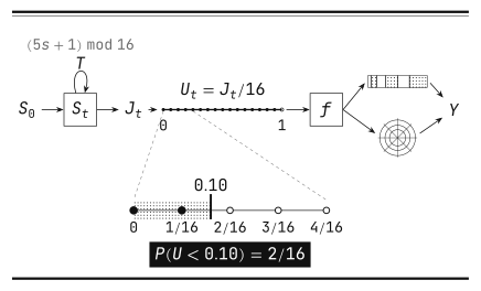
When I meet a new generative model, I like to ask where the randomness comes in and what happens once I fix it. If I’m trying to reproduce a sample, the seed is only part of the answer. Change the order in which the sampler uses the draws and the same seed can give me a different result.